Computational Chemistry
Molecular Dynamics I — From Newton's Equations to Ensembles
A practical introduction to molecular dynamics: equations of motion, Velocity Verlet, periodic boundaries, thermodynamic observables, RDF/VACF, force fields, constraints, thermostats, and barostats.
Lecture: Computational Chemistry
Instructor: YML (Young Min Rhee) Topic: Foundations of classical molecular dynamics
Molecular dynamics (MD) sounds almost suspiciously easy at first:
know where every atom is, know how fast it is moving, apply Newton, repeat until your laptop becomes a small space heater.
Formally, that is basically it. The actual pain begins when we ask for a trajectory that is numerically stable, physically meaningful, and long enough to tell us something useful rather than merely producing a very expensive atom screensaver.
This post develops the basic MD workflow from that viewpoint.
1. Molecular Dynamics as Deterministic Time Evolution
For particle $i$,
\[m_i \frac{d^2 \mathbf r_i}{dt^2} = \mathbf F_i = -\nabla_i U(\mathbf r_1,\ldots,\mathbf r_N).\]Once the potential-energy function $U$ is specified, the forces are known, and Newton’s equations determine the trajectory.
For $N$ particles in three dimensions, a microscopic state is represented by a point in a $6N$-dimensional phase space,
\[\Gamma = (\mathbf r_1,\ldots,\mathbf r_N, \mathbf p_1,\ldots,\mathbf p_N).\]This is the main distinction between MD and Monte Carlo (MC):
- MD generates a time-ordered, deterministic trajectory by integrating equations of motion.
- MC generates configurations through stochastic sampling rules.
The trajectory itself is usually not the prize. Nobody runs a 100 ns simulation just to admire frame 3,721,884 like it is modern art. What we usually want are statistical observables: energy, temperature, pressure, diffusion coefficients, structural correlations, free-energy differences, and so on.
If the system is ergodic, a time average can be related to an ensemble average,
\[\langle A \rangle = \lim_{\tau\rightarrow\infty} \frac{1}{\tau} \int_0^\tau A[\Gamma(t)]\,dt.\]In practice, simulations are finite. We therefore discard an initial equilibration interval and compute averages over the later production trajectory.
The goal of MD is generally not to predict the exact coordinates at a very long time. It is to generate statistically meaningful samples of a thermodynamic ensemble.
2. Why a Numerical Integrator Is Necessary
The first integrator everyone thinks of is Euler’s method. It is also the numerical equivalent of saying, “eh, close enough,” and then acting surprised when the total energy slowly walks out of the building.
A naive explicit Euler step is
\[\mathbf v(t+\Delta t) = \mathbf v(t)+\mathbf a(t)\Delta t,\] \[\mathbf r(t+\Delta t) = \mathbf r(t)+\mathbf v(t)\Delta t.\]In code:
a = F / m
v_next = v + a * dt
r_next = r + v * dt
This is cheap, but it accumulates significant numerical error and gives poor long-time energy conservation.
MD therefore uses integrators designed specifically for Newtonian dynamics.
3. Velocity Verlet
One of the standard choices is the Velocity Verlet algorithm.
First update the positions:
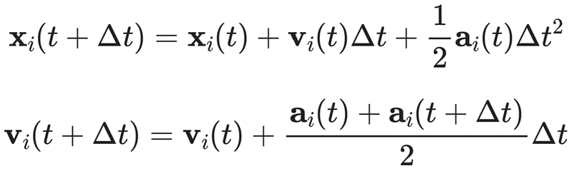
\[\mathbf r(t+\Delta t) = \mathbf r(t) + \mathbf v(t)\Delta t + \frac{1}{2}\mathbf a(t)\Delta t^2.\]Then evaluate the force at the new positions,
\[\mathbf F(t+\Delta t) = -\nabla U[\mathbf r(t+\Delta t)],\]and obtain the new acceleration,
\[\mathbf a(t+\Delta t) = \frac{\mathbf F(t+\Delta t)}{m}.\]Finally update the velocities:
\[\mathbf v(t+\Delta t) = \mathbf v(t) + \frac{1}{2} \left[ \mathbf a(t)+\mathbf a(t+\Delta t) \right] \Delta t.\]A compact Python implementation is:
def velocity_verlet(r, v, F, m, dt, force_fn):
    a = F / m[:, None]

    # 1. Update positions
    r_new = r + v * dt + 0.5 * a * dt**2

    # 2. Evaluate forces at the new positions
    F_new = force_fn(r_new)
    a_new = F_new / m[:, None]

    # 3. Update velocities
    v_new = v + 0.5 * (a + a_new) * dt

    return r_new, v_new, F_new
Velocity Verlet is popular because it manages to be boring in exactly the right way. It is:
- second-order accurate in time,
- time reversible,
- inexpensive,
- and reasonably stable for Hamiltonian dynamics.
Other common schemes include Leapfrog and Beeman integration. They differ in where positions and velocities are defined in time, their numerical stability, and how conveniently kinetic quantities are evaluated.
4. Periodic Boundary Conditions
A finite simulation box has artificial walls. For bulk liquid or solid simulations, we usually want the finite system to approximate a piece of an effectively infinite material.
Periodic boundary conditions (PBC) solve this by tiling space with copies of the simulation box.
For a cubic box of side length $L$, coordinates can be wrapped as
\[\mathbf r \leftarrow \mathbf r \bmod L.\]In two dimensions, one can think of opposite boundaries as being connected to form a torus. The same idea extends to three dimensions.
PBC gets rid of the embarrassing wall problem, but immediately creates a more sophisticated problem: every particle now has an infinite army of periodic clones.
For short-range interactions this is manageable. For Coulomb interactions, the clones unionize and demand to be included. That entire mess is the subject of Part II.
5. Temperature and Kinetic Energy
Temperature in classical MD is extracted from kinetic energy. In other words, the atoms are not carrying tiny thermometers; we infer temperature from how violently they are flying around.
The instantaneous kinetic energy is
\[K = \frac{1}{2} \sum_i m_i \mathbf v_i^2.\]Using equipartition,
\[T = \frac{2K}{N_{\mathrm{dof}}k_B},\]where $N_{\mathrm{dof}}$ is the number of active degrees of freedom.
E_kin = 0.5 * np.sum(m[:, None] * v**2)
T = 2 * E_kin / (dof * kB)
The precise number of degrees of freedom matters when center-of-mass motion or bond constraints have been removed.
6. Pressure and the Virial
For a classical system, the pressure can be estimated using the virial expression,
\[P = \frac{Nk_B T}{V} + \frac{1}{3V} \left\langle \sum_{i<j} \mathbf r_{ij}\cdot\mathbf F_{ij} \right\rangle.\]The first term is the ideal-gas contribution. The second term accounts for interparticle forces.
In an implementation, the pairwise virial contribution can be accumulated during force evaluation:
virial += np.dot(rij, fij)
7. Radial Distribution Function
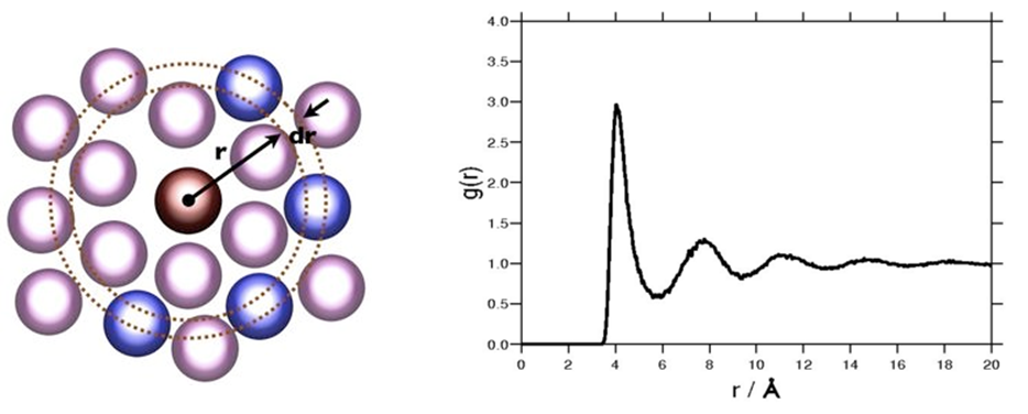
The radial distribution function, $g(r)$, measures how likely it is to find another particle at distance $r$ from a reference particle relative to an ideal gas at the same density.
For a homogeneous system,
\[g(r) = \frac{\text{observed number density at }r} {\text{ideal-gas number density at }r}.\]The spherical shell volume is approximately
\[dV = 4\pi r^2\,dr.\]A simulation therefore computes a histogram of pair distances and normalizes it by the expected number of particles in each shell.
hist = np.zeros(n_bins)

for frame in trajectory:
    for i in range(N):
        for j in range(i + 1, N):
            dr = frame[j] - frame[i]
            dr = minimum_image(dr, L)
            rij = np.linalg.norm(dr)

            bin_idx = int(rij / dr_bin)
            if bin_idx < n_bins:
                hist[bin_idx] += 2

r = np.arange(n_bins) * dr_bin
shell_volume = 4 * np.pi * r**2 * dr_bin
ideal_count = density * shell_volume * N * n_frames
g_r = hist / ideal_count
For liquid water, the O–O RDF shows where neighboring oxygens prefer to hang out. Peaks are basically the liquid saying, “yeah, around this distance is socially acceptable.”
8. Velocity Autocorrelation Function
Structural observables such as $g(r)$ tell us where particles like to sit. Dynamical observables ask a different question: does a particle remember what it was doing a moment ago, or has the liquid already ruined its plans?
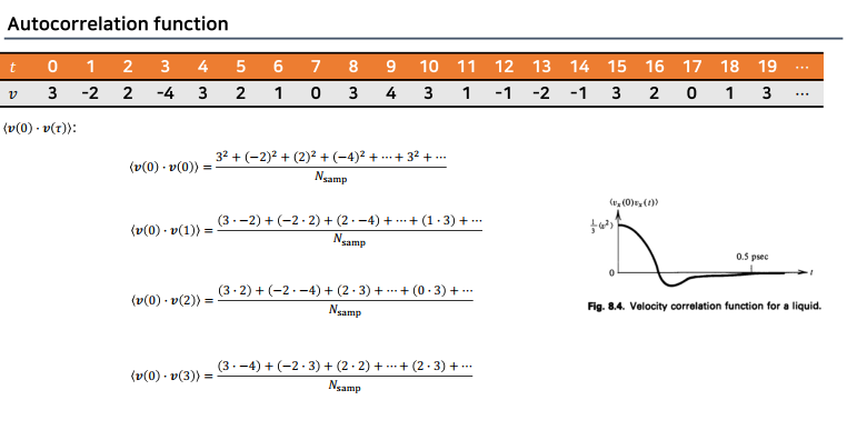
The velocity autocorrelation function (VACF) is
\[C_v(t) = \left\langle \mathbf v(0)\cdot\mathbf v(t) \right\rangle.\]A normalized form is
\[\widetilde C_v(t) = \frac{C_v(t)}{C_v(0)}.\]
Interpretation:
- rapid decay toward zero means the system loses velocity memory quickly;
- a long tail means motion remains correlated for longer;
- oscillations can indicate caging or vibrational dynamics.
A simple estimator is:
def vacf(vel_traj, max_lag):
    # vel_traj.shape == (n_frames, n_particles, 3)
    C = np.zeros(max_lag)

    for lag in range(max_lag):
        dots = []

        for t0 in range(len(vel_traj) - lag):
            dot = np.sum(
                vel_traj[t0] * vel_traj[t0 + lag],
                axis=1
            )
            dots.append(dot)

        C[lag] = np.mean(dots)

    return C / C[0]
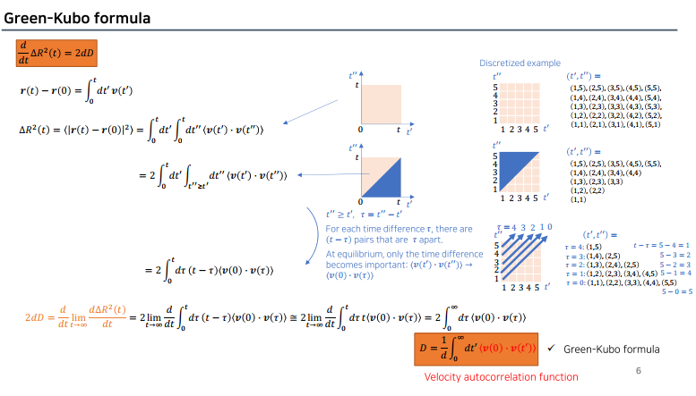
The VACF is also related to the self-diffusion coefficient through the Green–Kubo relation,
\[D = \frac{1}{3} \int_0^\infty C_v(t)\,dt.\]9. The Force Field Determines the Dynamics
At the classical level, an MD simulation is largely defined by its potential-energy function,
\[U(\mathbf r),\]because the forces follow from
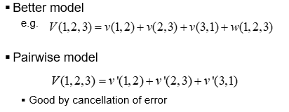
\[\mathbf F_i = -\nabla_i U.\]A force field is essentially a long list of agreements about how atoms are allowed to misbehave. A typical molecular-mechanics model separates the energy into bonded and non-bonded terms,
\[U = U_{\mathrm{bond}} + U_{\mathrm{angle}} + U_{\mathrm{dihedral}} + U_{\mathrm{improper}} + U_{\mathrm{vdW}} + U_{\mathrm{Coulomb}}.\]9.1 Bond stretching
A common approximation is a harmonic potential,
\[U_{\mathrm{bond}}(r) = \frac{1}{2}k_b(r-r_0)^2.\]9.2 Angle bending
Likewise,
\[U_{\mathrm{angle}}(\theta) = \frac{1}{2}k_\theta(\theta-\theta_0)^2.\]9.3 Dihedral torsions
A periodic form is often used,
\[U_{\mathrm{dihedral}}(\phi) = \sum_n k_n \left[ 1+\cos(n\phi-\delta_n) \right].\]Proper dihedrals describe torsional rotation, whereas improper terms are commonly used to preserve planarity or stereochemistry.
9.4 Coulomb interaction
For point charges,
\[U_{\mathrm{Coulomb}}(r_{ij}) = \frac{1}{4\pi\varepsilon_0} \frac{q_iq_j}{r_{ij}}.\]This $1/r$ decay is slow, which makes electrostatics under periodic boundary conditions nontrivial.
9.5 Lennard–Jones interaction
A standard model for short-range repulsion and dispersion is
\[U_{\mathrm{LJ}}(r) = 4\varepsilon \left[ \left(\frac{\sigma}{r}\right)^{12} - \left(\frac{\sigma}{r}\right)^6 \right].\]def lj_potential(r, epsilon, sigma):
sr6 = (sigma / r)**6
return 4 * epsilon * (sr6**2 - sr6)
def lj_force_mag(r, epsilon, sigma):
sr6 = (sigma / r)**6
return 24 * epsilon / r * (2 * sr6**2 - sr6)
10. Constraint Dynamics
Fast bond vibrations are numerically annoying because they force the time step to be tiny. X–H stretching, in particular, is the molecular-dynamics version of one hyperactive guy in the group project setting the schedule for everyone.
Fast bond vibrations impose a severe restriction on the time step.
For instance, X–H bond stretching occurs on a very short timescale. If those vibrations are integrated explicitly, $\Delta t$ must be small enough to resolve them.
A common alternative is to impose a holonomic constraint,
\[\sigma(\mathbf r) = |\mathbf r_i-\mathbf r_j|^2-d_{ij}^2 = 0.\]The constrained equations of motion can be written as
\[m_i\ddot{\mathbf r}_i = \mathbf F_i + \mathbf G_i,\]where $\mathbf G_i$ is a constraint force.
Using Lagrange multipliers,
\[\mathbf G_i = -\lambda \frac{\partial \sigma}{\partial \mathbf r_i}.\]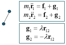
Algorithms such as SHAKE iteratively determine the multiplier so that the corrected coordinates satisfy the prescribed bond lengths after an unconstrained integration step.
The practical benefit is important: constraining high-frequency X–H stretching often allows a larger MD time step.
11. From NVE to NVT: Thermostats
Plain Newtonian dynamics with a time-independent Hamiltonian naturally corresponds to the microcanonical ensemble,
\[NVE: \qquad N,\;V,\;E=\text{constant}.\]To sample the canonical ensemble,
\[NVT: \qquad N,\;V,\;T=\text{constant},\]the dynamics must exchange energy with an effective heat bath.
The crudest thermostat is direct velocity rescaling: if the system is too hot, slow everyone down; if it is too cold, give everyone molecular espresso.
The simplest possible temperature correction is direct velocity rescaling,
\[\lambda = \sqrt{\frac{T_{\mathrm{target}}}{T_{\mathrm{current}}}}, \qquad \mathbf v_i \leftarrow \lambda\mathbf v_i.\]lambda_scale = np.sqrt(T_target / T_current)
v *= lambda_scale
This makes the displayed temperature look obedient, but statistical mechanics is not fooled that easily. Matching the number on the thermostat is not the same thing as sampling the canonical ensemble correctly.
More physically meaningful thermostat methods include:
- Andersen thermostat – random collisions with a heat bath;
- Langevin dynamics – friction plus stochastic noise;
- Nosé–Hoover / Nosé–Hoover chains – extended dynamical variables;
- stochastic velocity rescaling (Bussi thermostat) – canonical sampling with controlled temperature relaxation.
The important conceptual point is that a thermostat is not merely a device that keeps the displayed temperature at exactly $300\,\mathrm K$. Its purpose is to generate the desired thermodynamic ensemble.
12. NPT Dynamics and Barostats
For the isothermal–isobaric ensemble,
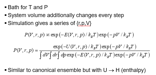
\[NPT: \qquad N,\;P,\;T=\text{constant},\]the simulation volume must also fluctuate.
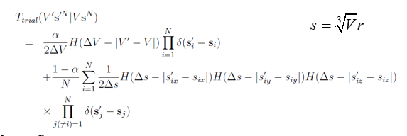
A barostat changes the box dimensions and rescales coordinates so that the system samples an appropriate pressure distribution.
Common approaches include:
- Berendsen pressure coupling,
- Andersen-type methods,
- Parrinello–Rahman dynamics,
- stochastic cell rescaling.
For anisotropic systems, the box need not change only in volume; its shape may also evolve.
13. Chaotic Trajectories Do Not Make MD Useless
MD trajectories exhibit Lyapunov instability: microscopic differences in initial conditions, floating-point arithmetic, compiler behavior, or hardware eventually grow into completely different trajectories.
So if two simulations start nearly identically and later one water molecule goes left while the other goes right, this is not evidence that one simulation became drunk. It is chaos doing its job.
Therefore, two nominally equivalent simulations may eventually produce completely different microscopic coordinates.
This does not imply that the simulation has failed. Exact long-time coordinates are not sacred; the statistics are.
The physically relevant comparison is usually statistical:
- average energy,
- temperature and pressure distributions,
- radial distribution functions,
- diffusion coefficients,
- free energies,
- structural populations,
- and other ensemble observables.
The exact long-time trajectory is fragile; the statistical distribution should be robust.
14. Practical MD Workflow
A minimal classical MD workflow can be summarized as:
- Choose a potential-energy model $U(\mathbf r)$.
- Compute forces using $\mathbf F=-\nabla U$.
- Integrate Newton’s equations with a stable scheme such as Velocity Verlet.
- Apply periodic boundary conditions.
- Use constraints when very fast bond vibrations are not of interest.
- Select a thermostat and/or barostat consistent with the target ensemble.
- Equilibrate the system.
- Run a production trajectory.
- Analyze ensemble observables rather than over-interpreting a single microscopic trajectory.
The next major complication is the treatment of non-bonded interactions under periodic boundary conditions, especially the slowly decaying Coulomb potential. That is the subject of Part II.