Computational Chemistry
Molecular Dynamics II — Cutoffs, Periodic Electrostatics, and Ewald Summation
Why short-range cutoffs work for Lennard-Jones interactions but fail for Coulomb electrostatics, and how Ewald summation resolves long-range interactions under periodic boundary conditions.
Lecture: Computational Chemistry
Instructor: YML (Young Min Rhee) Topic: Non-bonded interactions under periodic boundary conditions
Periodic boundary conditions remove artificial walls, which is great, but physics charges interest.
The moment we replicate the box periodically, every charge gets an infinite set of clones. Now a perfectly reasonable question becomes mathematically annoying:
how do we calculate interactions with infinitely many copies without waiting until the heat death of the universe?
A particle in the central simulation box does not interact only with the other particles in that box. Under PBC, it also has interactions with an infinite lattice of periodic images.
That is the central problem of this chapter:
How do we replace an infinite periodic interaction problem with a finite amount of computation without butchering the physics?
For rapidly decaying interactions, a real-space cutoff can work very well. For Coulomb electrostatics, a naive cutoff is generally not acceptable. The Ewald method solves this by transforming one difficult slowly convergent sum into several rapidly convergent terms.
1. Why $1/r$ and $1/r^6$ Behave Differently
Suppose an isotropic pair potential decays as
\[u(r)\propto \frac{1}{r^n}.\]The number of particles in a spherical shell of radius $r$ grows approximately as its area,
\[dN(r) \propto 4\pi r^2\,dr.\]A rough estimate of the contribution from that shell is therefore
\[dU(r) \propto r^2 \frac{1}{r^n}\,dr = r^{2-n}\,dr.\]The tail contribution beyond some radius $R$ behaves like
\[\int_R^\infty r^{2-n}\,dr.\]This immediately distinguishes short- and long-ranged interactions.
For the attractive part of Lennard–Jones,
\[u_{\mathrm{disp}}(r)\propto -\frac{1}{r^6},\]so the shell contribution decays as
\[r^{-4},\]which converges rapidly.
For Coulomb electrostatics,
\[u_{\mathrm C}(r) \propto \frac{1}{r},\]the corresponding shell factor scales as
\[r.\]A simple radial convergence argument therefore fails completely. Charge cancellation and global neutrality become essential, and the infinite lattice sum must be treated with much greater care.
This is why the sentence
“but the interaction is tiny when $r$ is large”
is not a valid argument by itself. There may be an absurd number of particles living at those large distances. One weak interaction times a ridiculous number of neighbors can still matter.
2. Real-Space Cutoffs
The most obvious idea is the computational equivalent of pretending distant relatives do not exist: choose a cutoff radius $r_c$ and ignore everything outside it.
\[u_{\mathrm{cut}}(r) = \begin{cases} u(r), & r<r_c,\\ 0, & r\ge r_c. \end{cases}\]
For a cubic periodic box of side length $L$, the usual minimum-image construction requires
\[r_c \le \frac{L}{2}.\]If the cutoff is larger than half the box length, the cutoff sphere can include multiple periodic images of the same physical particle.
3. Minimum Image Convention
For particles $i$ and $j$, define the displacement
\[\Delta\mathbf r_{ij} = \mathbf r_j-\mathbf r_i.\]Under the minimum image convention, each Cartesian component is mapped to the nearest periodic image,
\[\Delta r_\alpha \leftarrow \Delta r_\alpha - L_\alpha \operatorname{round} \left( \frac{\Delta r_\alpha}{L_\alpha} \right).\]For a cubic box:
def minimum_image(dr, L):
    return dr - L * np.round(dr / L)
The resulting vector gives the shortest separation between the two particles over all periodic images.
The minimum image convention is computationally convenient, but it is fundamentally a finite-range construction. It does not represent the full infinite electrostatic lattice.
4. Why Hard Truncation Is Problematic
Unfortunately, a hard cutoff is rude. The interaction exists one femtometer before $r_c$, then instantly disappears after crossing the line.
Mathematically, the potential is discontinuous at $r_c$,
\[\lim_{r\to r_c^-}u(r) \neq \lim_{r\to r_c^+}u(r).\]Since force is the negative derivative,
\[F(r) = -\frac{du}{dr},\]the discontinuity produces an impulsive or ill-defined force near the cutoff.
This can generate:
- poor energy conservation,
- artificial structural features,
- integration instability,
- and cutoff-dependent thermodynamic properties.
So instead of letting the potential fall off a cliff, practical force fields usually build it a little ramp.
5. Shifted Potential
A shifted potential subtracts the value at the cutoff,
\[u_{\mathrm{shift}}(r) = \begin{cases} u(r)-u(r_c), & r<r_c,\\ 0, & r\ge r_c. \end{cases}\]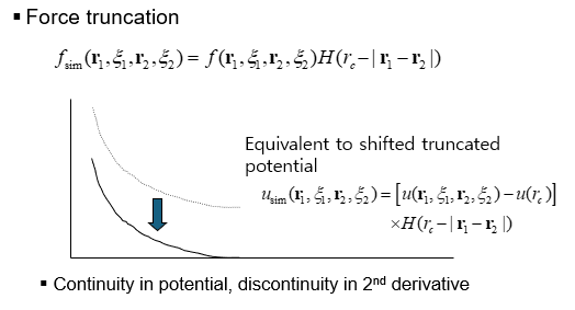
This guarantees
\[u_{\mathrm{shift}}(r_c)=0.\]Because the correction is a constant for $r<r_c$,
\[-\frac{d}{dr}[u(r)-u(r_c)] = -\frac{du}{dr},\]so the force inside the cutoff is unchanged.
However, the force generally remains discontinuous at $r_c$.
6. Switching Functions
A switching function gradually suppresses the interaction over an interval,
\[r_{\mathrm{on}} < r < r_c.\]A common construction is
\[u_{\mathrm{sw}}(r) = S(r)u(r),\]with
\[S(r)=1 \qquad (r\le r_{\mathrm{on}})\]and
\[S(r)=0 \qquad (r\ge r_c).\]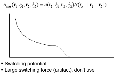
The force is then
\[F_{\mathrm{sw}}(r) = - \frac{d}{dr}[S(r)u(r)] = - S(r)\frac{du}{dr} - u(r)\frac{dS}{dr}.\]The second term is important: the switching function itself changes the force.
A well-designed switching polynomial can enforce continuity of both the potential and selected derivatives at the boundaries, but it also modifies the interaction over the switching region.
7. Force Switching
Instead of smoothing the potential first, one can construct a force that smoothly approaches zero,
\[F_{\mathrm{fs}}(r_c)=0,\]and then obtain a consistent potential by integration,
\[u_{\mathrm{fs}}(r) = -\int F_{\mathrm{fs}}(r)\,dr + C.\]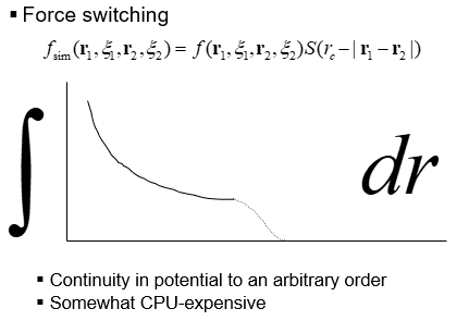
This is useful when force continuity is the primary numerical requirement. The price is that the original pair interaction is deliberately modified over a finite radial interval.
For rapidly decaying van der Waals interactions, these cutoff-based treatments can be well controlled. For electrostatics, the deeper problem remains: a local cutoff does not reproduce the infinite periodic Coulomb sum.
8. The Periodic Electrostatic Energy
Now comes the part where Lennard–Jones politely leaves the room and Coulomb electrostatics starts causing administrative problems.
For a finite nonperiodic system, the electrostatic energy is
\[U = \frac{1}{2} \sum_{i\ne j} \frac{q_iq_j} {4\pi\varepsilon_0 |\mathbf r_i-\mathbf r_j|}.\]Under periodic boundary conditions, every charge interacts with every periodic image.
Let
\[\mathbf n = (n_x,n_y,n_z) \in \mathbb Z^3\]label the image cells and let the box vectors define the lattice translation $\mathbf nL$.
The periodic electrostatic energy becomes
\[U_{\mathrm{PBC}} = \frac{1}{2} \frac{1}{4\pi\varepsilon_0} \sum_{i,j} \sum_{\mathbf n}^{\prime} \frac{q_iq_j} { |\mathbf r_i-\mathbf r_j+\mathbf nL| }.\]The prime means that the term
\[i=j,\qquad \mathbf n=\mathbf 0\]is excluded, because a point charge must not interact with itself in the original cell.
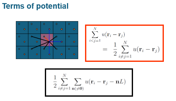
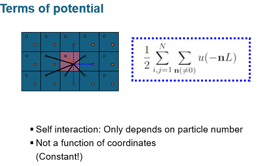
The bad news: this is an infinite lattice sum with painfully slow convergence. Worse, in three dimensions it is conditionally convergent, meaning that even the order in which you sum things matters unless the boundary convention is specified. Electrostatics has now become a bureaucracy.
A charge-neutral simulation cell,
\[\sum_i q_i=0,\]is normally required for the standard periodic Ewald treatment.
9. The Key Ewald Idea
Ewald’s trick is one of those ideas that looks slightly unhinged until you realize it is exact.
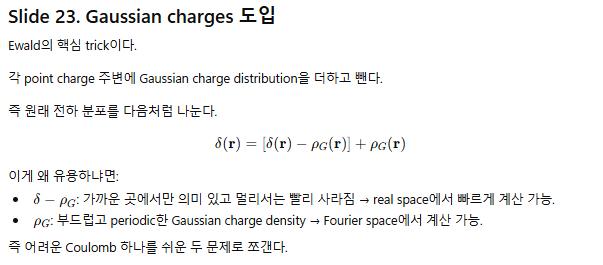
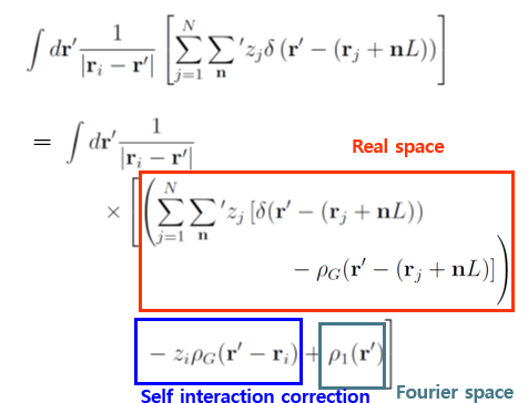
We deliberately add a Gaussian screening charge around every point charge, solve the easier screened problem, then compensate for the thing we just added. In short:
add fake charge, make the math easier, subtract the fake charge, pretend this was obvious all along.
Formally, the Ewald method introduces a Gaussian screening distribution around each point charge.
The fundamental identity is
\[\frac{1}{r} = \frac{\operatorname{erfc}(\alpha r)}{r} + \frac{\operatorname{erf}(\alpha r)}{r},\]where $\alpha$ is the Ewald splitting parameter.
This identity is exact. No physics has been approximated yet; we have only reorganized the problem into two pieces that are computationally less awful.
The two pieces have very different numerical properties.
Short-range part
\[\frac{\operatorname{erfc}(\alpha r)}{r}\]decays rapidly in real space.
Smooth long-range part
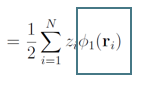
\[\frac{\operatorname{erf}(\alpha r)}{r}\]is smooth and slowly varying, making it efficient to represent in reciprocal space with a Fourier series.
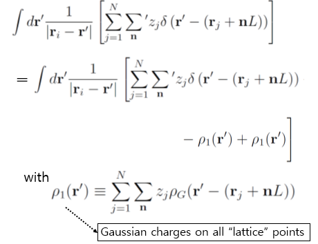
So instead of wrestling one giant cursed sum, Ewald summation splits the job into several well-behaved pieces:
\[U_{\mathrm{Ewald}} = U_{\mathrm{real}} + U_{\mathrm{reciprocal}} + U_{\mathrm{self}} + U_{\mathrm{surface}},\]where the final surface term depends on the chosen macroscopic boundary condition and is often zero under conducting (“tin-foil”) boundary conditions.
10. Real-Space Ewald Term
The screened real-space contribution is
\[U_{\mathrm{real}} = \frac{1}{2} \frac{1}{4\pi\varepsilon_0} \sum_{i,j} \sum_{\mathbf n}^{\prime} q_iq_j \frac{ \operatorname{erfc} \left( \alpha |\mathbf r_{ij}+\mathbf nL| \right) } { |\mathbf r_{ij}+\mathbf nL| }.\]Because
\[\operatorname{erfc}(\alpha r) \rightarrow 0\]rapidly with increasing $r$, this term can be truncated in real space.

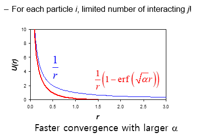
This is the crucial improvement: the original unscreened $1/r$ interaction was long-ranged, but the screened real-space interaction is short-ranged.
11. Reciprocal-Space Ewald Term
The smooth Gaussian charge distribution is periodic, so it can be expanded in reciprocal-lattice vectors $\mathbf k$.
For an orthorhombic periodic cell,
\[\mathbf k = 2\pi \left( \frac{m_x}{L_x}, \frac{m_y}{L_y}, \frac{m_z}{L_z} \right), \qquad m_x,m_y,m_z\in\mathbb Z.\]Define the charge structure factor
\[S(\mathbf k) = \sum_j q_j e^{i\mathbf k\cdot\mathbf r_j}.\]Then the reciprocal-space energy can be written as
\[U_{\mathrm{reciprocal}} = \frac{1}{2V\varepsilon_0} \sum_{\mathbf k\ne 0} \frac{ e^{-k^2/(4\alpha^2)} }{ k^2 } \left| S(\mathbf k) \right|^2.\]Equivalent forms often factor out $1/(4\pi\varepsilon_0)$; the exact prefactor therefore depends on the electrostatic unit convention being used.
The exponential factor
\[e^{-k^2/(4\alpha^2)}\]causes rapid convergence in reciprocal space.
12. Self-Interaction Correction
Of course, after inventing fake Gaussian charge clouds, we inherit a fake self-interaction too. Ewald giveth, Ewald taketh away.
Introducing Gaussian screening creates an artificial interaction between each point charge and its own compensating Gaussian.
That contribution must be removed.
The self-energy correction is
\[U_{\mathrm{self}} = - \frac{\alpha} {\sqrt{\pi}} \frac{1}{4\pi\varepsilon_0} \sum_i q_i^2.\]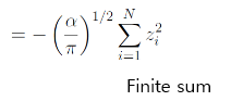
This term depends on the charges and on $\alpha$, but not on particle separations.
It exists purely because of the Ewald decomposition.
13. What Does the Ewald Parameter $\alpha$ Do?
The splitting parameter $\alpha$ does not change the exact electrostatic energy when both sums are converged.
It only changes how the computational work is divided.
Large $\alpha$:
- makes $\operatorname{erfc}(\alpha r)$ decay faster,
- reduces the required real-space cutoff,
- but requires more reciprocal-space resolution.
Small $\alpha$:
- makes the real-space term longer ranged,
- but makes the reciprocal-space term converge with fewer modes.
Therefore, $\alpha$, the real-space cutoff, and the reciprocal-space cutoff are tuning parameters for accuracy and performance.
14. From Ewald to Particle Mesh Ewald
Direct Ewald works, but for large systems the reciprocal-space part starts asking for unreasonable amounts of compute. Enter PME, whose main superpower is saying: “what if we let FFT do the boring part?”
Particle Mesh Ewald (PME) accelerates the reciprocal-space calculation by:
- assigning particle charges to a mesh,
- solving the reciprocal-space electrostatics on that grid,
- using FFTs,
- interpolating forces back to particle positions.
The resulting scaling is approximately
\[\mathcal O(N\log N),\]which is why PME is widely used in biomolecular and condensed-phase MD.
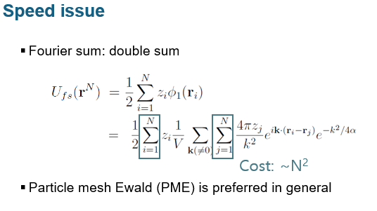
The underlying physics is still Ewald splitting; PME is primarily an algorithmic acceleration of the reciprocal-space term.
15. Short-Range vs. Long-Range Interactions
At this point the short-range/long-range distinction stops being a vague textbook slogan and becomes a very practical rule.
Lennard–Jones / dispersion
The attractive tail behaves as
\[r^{-6},\]so real-space cutoff methods are often accurate when combined with appropriate switching, shifting, and sometimes analytical long-range corrections.
Coulomb electrostatics
The potential behaves as
\[r^{-1}.\]Its periodic contribution depends collectively on a very large set of charges and images. A naive cutoff changes the physics and can strongly affect structure, energetics, dielectric response, and transport properties.
For periodic condensed-phase systems, lattice-summation methods such as Ewald or PME are therefore standard.
16. Conceptual Summary
The logic of periodic non-bonded interactions is:
\[\text{PBC} \Longrightarrow \text{infinite periodic images}\] \[\Downarrow\] \[\text{Can the interaction be safely localized?}\]For rapidly decaying interactions:
\[r^{-6} \Longrightarrow \text{real-space cutoff is often practical}.\]For Coulomb interactions:
\[r^{-1} \Longrightarrow \text{naive truncation is unreliable}.\]Ewald summation resolves this by using the exact decomposition
\[\frac{1}{r} = \frac{\operatorname{erfc}(\alpha r)}{r} + \frac{\operatorname{erf}(\alpha r)}{r},\]which turns the problem into:
\[\boxed{ \text{short-range real-space sum} + \text{smooth reciprocal-space sum} - \text{self interaction} }\]with a possible boundary-condition-dependent surface term.
That decomposition is the conceptual bridge from a formally infinite Coulomb lattice to an efficient periodic electrostatics algorithm.